Last updated: 2019-03-06
workflowr checks: (Click a bullet for more information)-
✔ R Markdown file: up-to-date
Great! Since the R Markdown file has been committed to the Git repository, you know the exact version of the code that produced these results.
-
✔ Environment: empty
Great job! The global environment was empty. Objects defined in the global environment can affect the analysis in your R Markdown file in unknown ways. For reproduciblity it’s best to always run the code in an empty environment.
-
✔ Seed:
set.seed(20190211)The command
set.seed(20190211)was run prior to running the code in the R Markdown file. Setting a seed ensures that any results that rely on randomness, e.g. subsampling or permutations, are reproducible. -
✔ Session information: recorded
Great job! Recording the operating system, R version, and package versions is critical for reproducibility.
-
Great! You are using Git for version control. Tracking code development and connecting the code version to the results is critical for reproducibility. The version displayed above was the version of the Git repository at the time these results were generated.✔ Repository version: b7d812d
Note that you need to be careful to ensure that all relevant files for the analysis have been committed to Git prior to generating the results (you can usewflow_publishorwflow_git_commit). workflowr only checks the R Markdown file, but you know if there are other scripts or data files that it depends on. Below is the status of the Git repository when the results were generated:
Note that any generated files, e.g. HTML, png, CSS, etc., are not included in this status report because it is ok for generated content to have uncommitted changes.Ignored files: Ignored: .Rhistory Ignored: .Rproj.user/ Untracked files: Untracked: code/alldata_compiler.R Untracked: code/contab_maker.R Untracked: code/mut_excl_genes_datapoints.R Untracked: code/mut_excl_genes_generator.R Untracked: code/quadratic_solver.R Untracked: code/simresults_generator.R Untracked: data/All_Data_V2.csv Untracked: data/alkati_growthcurvedata.csv Untracked: data/alkati_growthcurvedata_popdoublings.csv Untracked: data/alkati_melanoma_vemurafenib_figure_data.csv Untracked: data/all_data.csv Untracked: data/tcga_luad_expression/ Untracked: data/tcga_skcm_expression/ Untracked: docs/figure/Filteranalysis.Rmd/ Untracked: docs/figure/baf3_alkati_transformations.Rmd/ Untracked: output/alkati_filtercutoff_allfilters.csv Untracked: output/alkati_luad_exonimbalance.pdf Untracked: output/alkati_mtn_pval_fig2B.pdf Untracked: output/alkati_skcm_exonimbalance.pdf Untracked: output/all_data_luad.csv Untracked: output/all_data_luad_egfr.csv Untracked: output/all_data_skcm.csv Untracked: output/baf3_alkati_figure_deltaadjusted_doublings.pdf Untracked: output/baf3_barplot.pdf Untracked: output/baf3_elisa_barplot.pdf Untracked: output/egfr_luad_exonimbalance.pdf Untracked: output/fig2b2_filtercutoff_atinras_totalalk.pdf Untracked: output/fig2b_filtercutoff_atibraf.pdf Untracked: output/fig2b_filtercutoff_atinras.pdf Untracked: output/luad_alk_exon_expression.csv Untracked: output/luad_egfr_exon_expression.csv Untracked: output/melanoma_vemurafenib_fig.pdf Untracked: output/skcm_alk_exon_expression.csv
Expand here to see past versions:
| tle: “ALKATI Filter Cutoff Analysis” |
| thor: “Haider Inam” |
| te: “2/18/2019” |
| tput: html_document |
library(ggplot2)
library(knitr)
library(dplyr)
Attaching package: 'dplyr'The following objects are masked from 'package:stats':
filter, lagThe following objects are masked from 'package:base':
intersect, setdiff, setequal, unionlibrary(tictoc)
library(foreach)
library(doParallel)Loading required package: iteratorsLoading required package: parallelsource("code/alldata_compiler.R")
source("code/contab_maker.R")
######################Cleanup for GGPlot2#########################################
cleanup=theme_bw() +
theme(plot.title = element_text(hjust=.5),
panel.grid.major = element_blank(),
panel.grid.major.y = element_blank(),
panel.background = element_blank(),
axis.line = element_line(color = "black"))Varying Filter for mean RPKM from 1:100
Note that by mean RPKM, I mean ratio of 20-29 RPKM/1-19 RPKM
#Run Filter Analysis
ct=1
simresults<-matrix(nrow=100,ncol=2)
alldata=read.csv("data/all_data.csv",sep=",",header=T,stringsAsFactors=F)
for (meanRPKM in 1:100){
  alldata_filtered=alldata%>%
    group_by(Patid,mean_RPKM_1.19,mean_RPKM_20.29,Ratio20.29, mRNA_count,BRAF,NRAS,RSEM_normalized)%>%
    summarize(ATI=as.numeric(mRNA_count>=500&Ratio20.29>meanRPKM&RSEM_normalized>=100)[1])

  alldata_comp=alldata_compiler(alldata_filtered,'BRAF','NRAS','ATI','N',"N/A","N/A")[[2]]

  contab_pc1_genex=contab_maker(alldata_comp$Positive_Ctrl1,alldata_comp$genex,alldata_comp)
  simresults[ct,1]=ct #Total Count
  simresults[ct,2]=fisher.test(contab_pc1_genex)$p.value #p.value
  ct=ct+1
}
count=simresults[c(1:100),1]
pval=simresults[c(1:100),2]
colnames(simresults)=c("totCt","p_val")
cols=c("totCt","p_val")

simresults=as.data.frame(simresults, stringsAsFactors = F, )
simresults[colnames(simresults)] <- lapply(simresults[colnames(simresults)],as.character)
simresults[colnames(simresults)] <- lapply(simresults[colnames(simresults)],as.numeric)

#Plot Results
ggplot(simresults,aes(x=totCt,y=p_val))+geom_line(size=3)+ggtitle("Varying RPKM Filter")+xlab("Exon20:29/Exon1:19")+ylab("P-value")+theme_bw()+theme(plot.title = element_text(hjust=.5),text = element_text(size=30,face="bold"),axis.title = element_text(face="bold",size="26"),axis.text=element_text(face="bold",size="26"))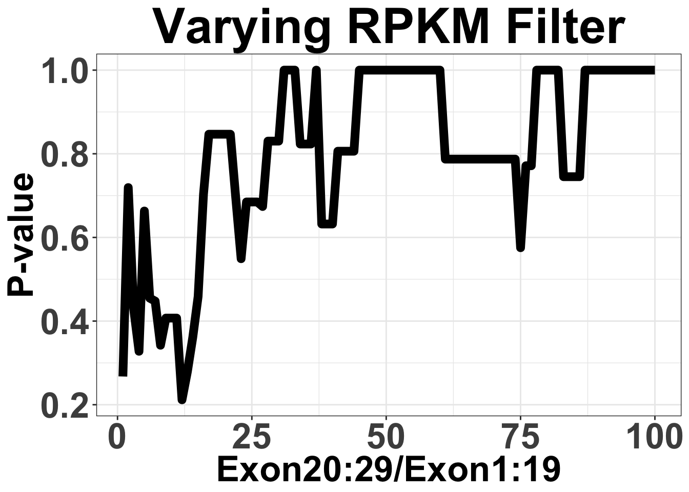
Expand here to see past versions of unnamed-chunk-2-1.png:
| Version | Author | Date |
|---|---|---|
| 4b082e4 | haiderinam | 2019-02-19 |
# ggsave("filteranalysis_RPKM.pdf",width = 9,height = 6,units = "in",useDingbats=F)Varying Filter for mean RSEM from 1 to 1000
Note that these are the sum of RSEM across all ALK-exons
#Run Filter Analysis
ct=1
simresults<-matrix(nrow=1000,ncol=2)
alldata=read.csv("data/all_data.csv",sep=",",header=T,stringsAsFactors=F)
for (rsem in 1:1000){
  alldata_filtered=alldata%>%
    group_by(Patid,mean_RPKM_1.19,mean_RPKM_20.29,Ratio20.29, mRNA_count,BRAF,NRAS,RSEM_normalized)%>%
    summarize(ATI=as.numeric(mRNA_count>=500&Ratio20.29>10&RSEM_normalized>=rsem)[1])
  alldata_comp=alldata_compiler(alldata_filtered,'BRAF','NRAS','ATI','N',"N/A","N/A")[[2]]

  contab_pc1_genex=contab_maker(alldata_comp$Positive_Ctrl1,alldata_comp$genex,alldata_comp)
  simresults[ct,1]=ct #Total Count
  simresults[ct,2]=fisher.test(contab_pc1_genex)$p.value #p.value
  ct=ct+1
}
count=simresults[c(1:100),1]
pval=simresults[c(1:100),2]
colnames(simresults)=c("totCt","p_val")
cols=c("totCt","p_val")

simresults=as.data.frame(simresults, stringsAsFactors = F, )
simresults[colnames(simresults)] <- lapply(simresults[colnames(simresults)],as.character)
simresults[colnames(simresults)] <- lapply(simresults[colnames(simresults)],as.numeric)

#Plot Results
ggplot(simresults,aes(x=totCt,y=p_val))+geom_line(size=3)+ggtitle("Varying RSEM Filter")+xlab("RSEM")+ylab("P-Value")+theme_bw()+theme(plot.title = element_text(hjust=.5),text = element_text(size=30,face="bold"),axis.title = element_text(face="bold",size="26"),axis.text=element_text(face="bold",size="26"))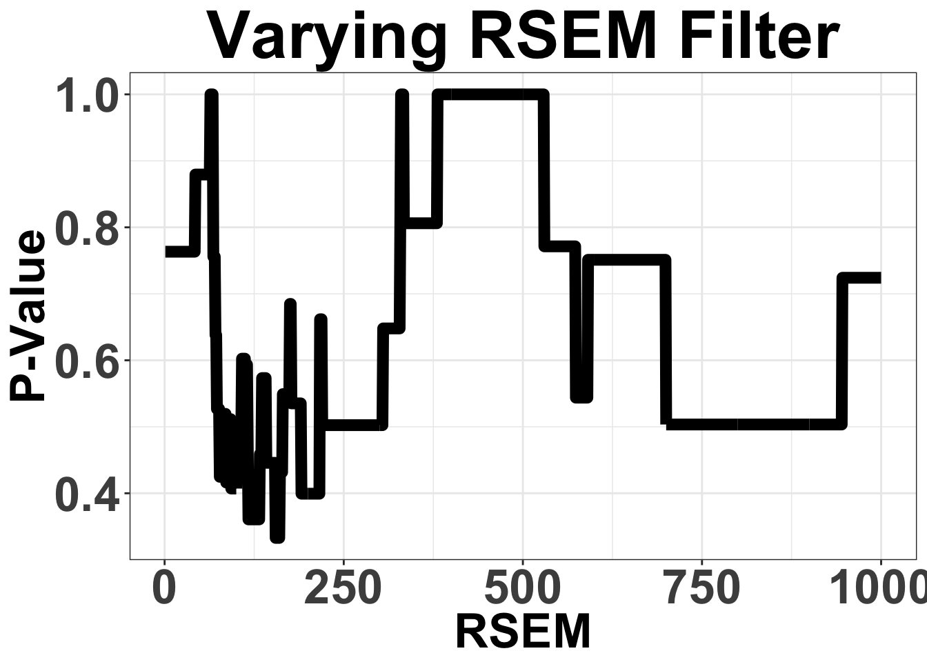
Expand here to see past versions of unnamed-chunk-3-1.png:
| Version | Author | Date |
|---|---|---|
| 4b082e4 | haiderinam | 2019-02-19 |
# ggsave("filteranalysis_RSEM.pdf",width = 9,height = 6,units = "in",useDingbats=F)Varying Filter for ALK raw read count from 1 to 10,000
Note that these are the sum of mRNA counts across all ALK-exons
#Run Filter Analysis
ct=1
simresults<-matrix(nrow=1000,ncol=2)
alldata=read.csv("data/all_data.csv",sep=",",header=T,stringsAsFactors=F)
for (rawreadcount in 1:1000){
  alldata_filtered=alldata%>%
    group_by(Patid,mean_RPKM_1.19,mean_RPKM_20.29,Ratio20.29, mRNA_count,BRAF,NRAS,RSEM_normalized)%>%
    summarize(ATI=as.numeric(mRNA_count>=rawreadcount&Ratio20.29>10&RSEM_normalized>=100)[1])
  alldata_comp=alldata_compiler(alldata_filtered,'BRAF','NRAS','ATI','N',"N/A","N/A")[[2]]

  contab_pc1_genex=contab_maker(alldata_comp$Positive_Ctrl1,alldata_comp$genex,alldata_comp)

  simresults[ct,1]=ct #Total Count
  simresults[ct,2]=fisher.test(contab_pc1_genex)$p.value #p.value
  ct=ct+1
  }
count=simresults[c(1:100),1]
pval=simresults[c(1:100),2]
colnames(simresults)=c("totCt","p_val")

simresults=as.data.frame(simresults, stringsAsFactors = F, )
simresults[colnames(simresults)] <- lapply(simresults[colnames(simresults)],as.character)
simresults[colnames(simresults)] <- lapply(simresults[colnames(simresults)],as.numeric)

#Plot results
ggplot(simresults,aes(x=totCt,y=p_val))+geom_line(size=3)+ggtitle("Varying ALK Raw Read Count")+xlab("Count")+ylab("P-value")+theme_bw()+theme(plot.title = element_text(hjust=.5),text = element_text(size=30,face="bold"),axis.title = element_text(face="bold",size="26"),axis.text=element_text(face="bold",size="26"))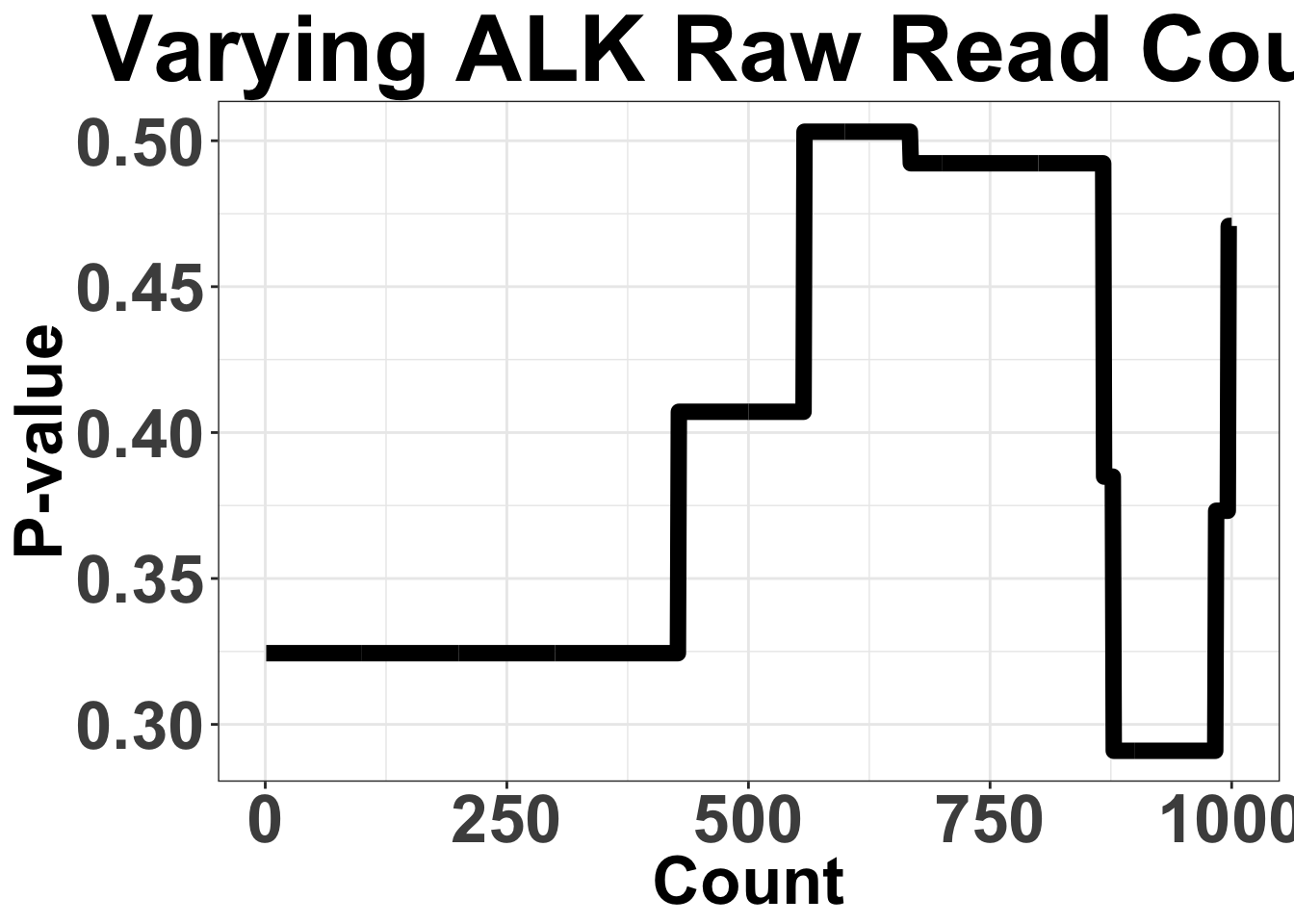
Expand here to see past versions of unnamed-chunk-4-1.png:
| Version | Author | Date |
|---|---|---|
| 4b082e4 | haiderinam | 2019-02-19 |
# ggsave("filteranalysis_Count.pdf",width = 9,height = 6,units = "in",useDingbats=F)Varying all Filters. This runs on parallel for-loops to improve computation time.
Since the filter cutoffs code take a long time, it is only run once. This code generates alkati_filtercutoff_allfilters.csv
#This chunk utilizes parallel for-loops to omptimize computational efficiency
#Run Filter Analysis using combination of filters
tic()
filename="data/all_data.csv"
alldata=read.csv(filename,sep=",",header=T,stringsAsFactors=F)

cores=detectCores()
cl= makeCluster(cores[1]-1)
registerDoParallel(cl)

#RPKM read count 1 to 100
simresults<-foreach(rawreadcount=seq(from=1,to=1500,by=10),.combine = rbind) %dopar% {
ct=1
simresults=matrix(nrow=100000,ncol=7)
library(dplyr)
#RSEM read count 1 to 1000
  for (rsem in seq(from=1,to=1000,by=10)){
    #Raw  read count 1 to 10,000
    for (rpkm in seq(from=2,to=30,by=2)) {

      alldata_filtered=alldata%>%
        group_by(Patid,mean_RPKM_1.19,mean_RPKM_20.29,Ratio20.29, mRNA_count,BRAF,NRAS,RSEM_normalized)%>%
        summarize(ATI=as.numeric(mRNA_count>=rawreadcount&Ratio20.29>=rpkm&RSEM_normalized>=rsem)[1])
      alldata_comp=alldata_compiler(alldata_filtered,'BRAF','NRAS','ATI','N',"N/A","N/A")[[2]]

      contab_pc1_genex=contab_maker(alldata_comp$Positive_Ctrl1,alldata_comp$genex,alldata_comp)
      contab_pc2_genex=contab_maker(alldata_comp$Positive_Ctrl2,alldata_comp$genex,alldata_comp)
      tot_alkati=sum(alldata_comp$genex)
      simresults[ct,1]=ct #Totalcount
      simresults[ct,2]=rpkm #RPKM
      simresults[ct,3]=rsem #RSEM
      simresults[ct,4]=rawreadcount #Alkreads
      simresults[ct,5]=fisher.test(contab_pc1_genex)$p.value #p.value
      simresults[ct,6]=fisher.test(contab_pc2_genex)$p.value #p.value
      simresults[ct,7]=tot_alkati #Total count of ALKATI patients
      ct=ct+1
    }
  }
simresults
}
stopCluster(cl)
toc()
  colnames(simresults)=c("totCt","rpkm","rsem","alkreads","p_val_pc1","p_val_pc2","tot_alk")

  #making simresults a dataframe
  simresults=as.data.frame(simresults, stringsAsFactors = F)
  #making everything a numeric
simresults[colnames(simresults)] <- lapply(simresults[colnames(simresults)],as.character)
simresults[colnames(simresults)] <- lapply(simresults[colnames(simresults)],as.numeric)

# write.csv(simresults,"output/alkati_filtercutoff_allfilters.csv")simresults=read.csv("output/alkati_filtercutoff_allfilters.csv")Figure 3a
NRAS vs ALKATI
Heat map for NRAS vs ALKATI P-values are only shown if there were at least 20 patients that met those filters
datapoints=simresults %>%
  filter(rsem<=500,alkreads<=1500)%>%
  group_by(rsem,alkreads,tot_alk) %>%
  summarise(min_p_val_pc2=min(p_val_pc2),rpkm_atpval=rpkm[min(p_val_pc2)][1])
datapoints[datapoints$tot_alk<20,]$min_p_val_pc2=""
datapoints$min_p_val_pc2=as.numeric(datapoints$min_p_val_pc2)

ggplot(datapoints,aes(x=alkreads,y=rsem))+geom_tile(aes(fill=min_p_val_pc2))+
      scale_fill_gradient2(low ="red" ,mid ="white" ,high ="blue",midpoint = .4 ,name="P-Value", na.value = "gray",guide = "legend",breaks=c(.1,.2,.4,.6,.8,1))+
      theme(panel.grid.major = element_blank(),
            panel.grid.minor = element_blank(),
            panel.background = element_blank(),
            axis.line = element_line(colour = "black"))+
      xlab("Number of ALK Reads")+ylab("RSEM")+
      # ggtitle("Varying Combinations of Filters Does Not Create \nMutual Exclusivity Between ALK-ATI & BRAF")+
      theme_bw()+
      theme(plot.title = element_text(hjust=.5),text = element_text(size=30,face="bold"),axis.title = element_text(face="bold",size="26"),axis.text=element_text(face="bold",color="black",size="26"))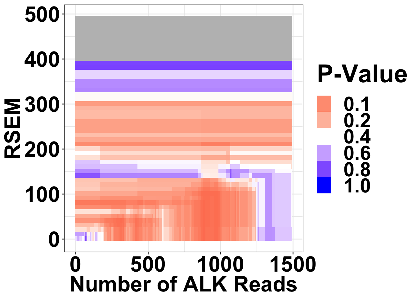
Expand here to see past versions of unnamed-chunk-7-1.png:
| Version | Author | Date |
|---|---|---|
| 0b5f5cb | haiderinam | 2019-02-19 |
| 4b082e4 | haiderinam | 2019-02-19 |
ggsave("output/fig2b_filtercutoff_atinras.pdf",width = 16,height = 14,units = "in",useDingbats=F)
###Regions with less than 20 patients are shaded gray.

ggplot(datapoints,aes(x=alkreads,y=rsem))+geom_tile(aes(fill=tot_alk))+
  scale_fill_gradient(,low="white",high="red",breaks = c(0,5,10,25,50,75,100),limits=c(0,100),name="ALKATI \nPatients \ndetected",guide = "legend",na.value = "red")+
  cleanup+
  theme(panel.grid.major = element_blank(),
            panel.grid.minor = element_blank(),
            panel.background = element_blank(),
            axis.line = element_line(colour = "black"))+
      xlab("Number of ALK Reads")+ylab("RSEM")+
      theme_bw()+
      theme(plot.title = element_text(hjust=.5),text = element_text(size=30,face="bold"),axis.title = element_text(face="bold",size="26"),axis.text=element_text(face="bold",color="black",size="26"))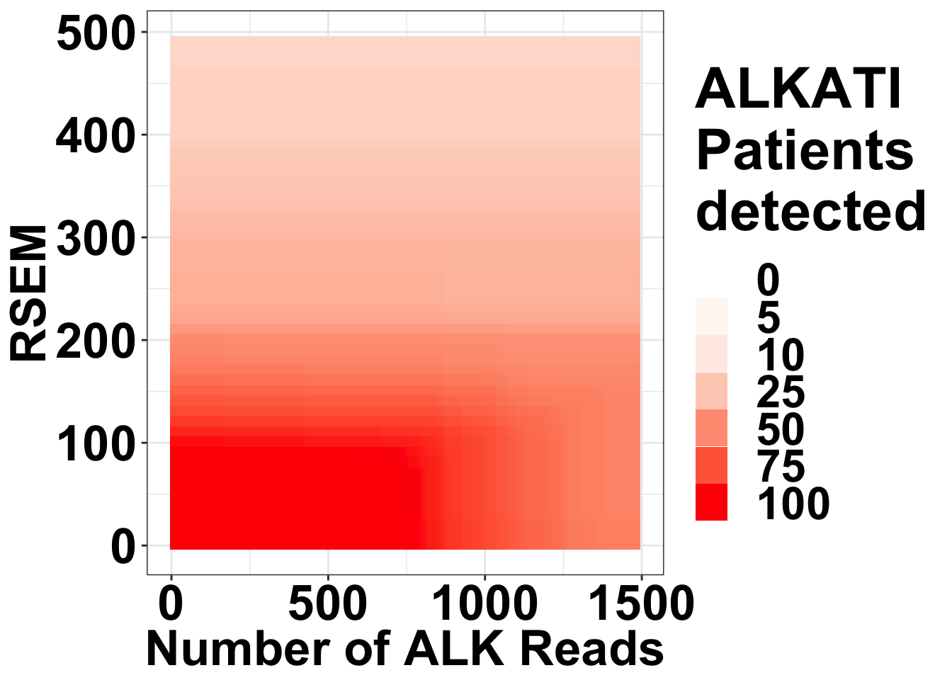
Expand here to see past versions of unnamed-chunk-7-2.png:
| Version | Author | Date |
|---|---|---|
| 0b5f5cb | haiderinam | 2019-02-19 |
# ggsave("output/fig2b2_filtercutoff_atinras_totalalk.pdf",width = 16,height = 14,units = "in",useDingbats=F)Heat map for NRAS vs ALKATI with count data
datapoints=simresults %>%
  filter(rsem<=500,alkreads<=1000)%>%
  group_by(rsem,alkreads,tot_alk) %>%
  summarise(min_p_val_pc2=min(p_val_pc2),rpkm_atpval=rpkm[min(p_val_pc2)][1])

  ggplot(datapoints,aes(x=alkreads,y=rsem))+geom_tile(aes(fill=tot_alk))+
    scale_fill_gradient2(low ="red" ,mid ="white" ,midpoint = 40,high ="blue",name="ALKATI Count")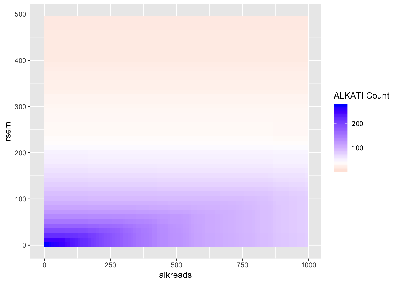
Expand here to see past versions of unnamed-chunk-8-1.png:
| Version | Author | Date |
|---|---|---|
| 4b082e4 | haiderinam | 2019-02-19 |
#Trying different tiles for RPKM
datapoints=simresults %>%
filter(rsem<=500,alkreads<=2000,rpkm%in%c(6,12,18,30))%>%
group_by(rsem,alkreads,tot_alk,rpkm) %>%
summarise(min_p_val_pc2=min(p_val_pc2))

ggplot(datapoints,aes(x=alkreads,y=rsem))+geom_tile(aes(fill=tot_alk))+facet_wrap(~rpkm)+
  scale_fill_gradient2(low ="red" ,mid ="white" ,midpoint = 40,high ="blue",name="ALKATI Count")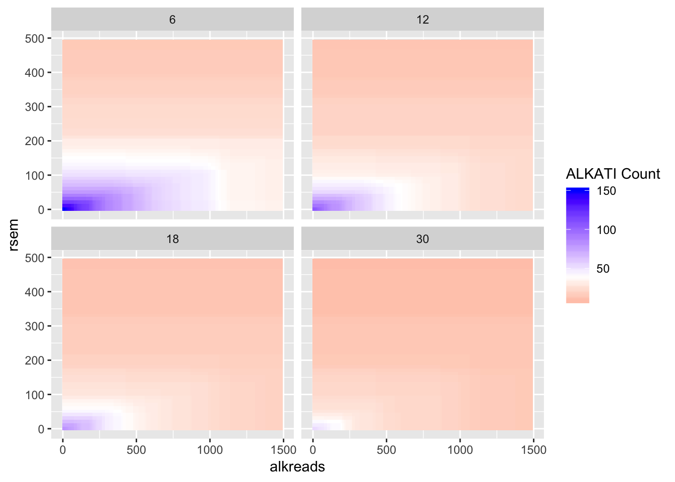
Expand here to see past versions of unnamed-chunk-8-2.png:
| Version | Author | Date |
|---|---|---|
| 4b082e4 | haiderinam | 2019-02-19 |
###Distribution of the number of ALKATI patients across different conditions
###Remember: ALKATI patients had exon ratio of 10, rsem >100, and counts >500. i.e. green region
###The takeaway from this plot is that we can try most filters without having to worry about patient numbers. Will look at the p-values for these orange filters next
ggplot(datapoints,aes(x=alkreads,y=rsem))+geom_tile(aes(fill=tot_alk))+facet_grid(~rpkm)+
  scale_fill_gradientn(colours = rainbow(5),values=c(.1,.2,.3,.4,1),limits=c(0,100),breaks = c(9,10,20,30,40,100),name="# ALKATI \n Patients",guide = "legend")+
  ggtitle("Total ALKATI patients across exon20-29/ex1-19 ratios")+
  cleanup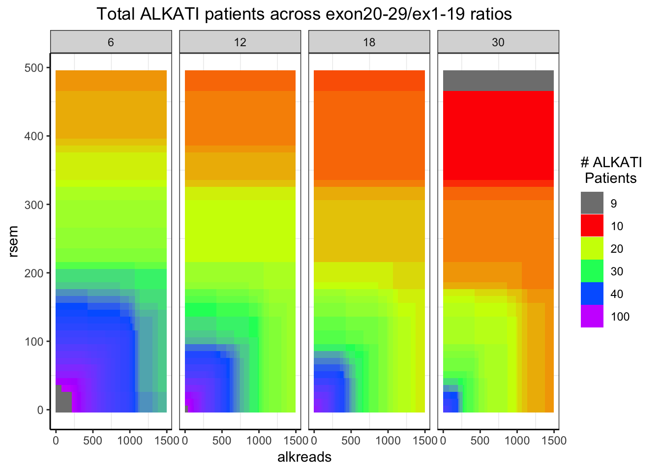
Expand here to see past versions of unnamed-chunk-8-3.png:
| Version | Author | Date |
|---|---|---|
| 4b082e4 | haiderinam | 2019-02-19 |
###Taking a look at whether there are any statistically significant regions.
###There is only one region. We don't see mutual exclusivity at this region in the p-value plot
###only p-values between 0 and 0.1 are shown
ggplot(datapoints,aes(x=alkreads,y=rsem))+geom_tile(aes(fill=min_p_val_pc2))+facet_grid(~rpkm)+
  scale_fill_gradient2(low ="red" ,mid ="white" ,high ="blue",midpoint = .05 ,name="P-Value",guide = "legend",limits=c(0,.1))+
  cleanup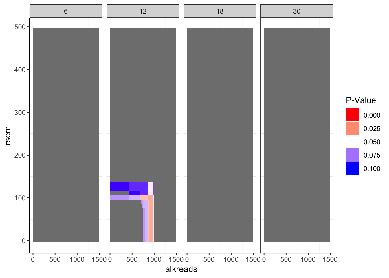
Expand here to see past versions of unnamed-chunk-8-4.png:
| Version | Author | Date |
|---|---|---|
| 4b082e4 | haiderinam | 2019-02-19 |
###If there are <20 patients for a set of filters, take that data out.

datapoints[datapoints$tot_alk<20,]$min_p_val_pc2=""
datapoints$min_p_val_pc2=as.numeric(datapoints$min_p_val_pc2)

###Regions with less than 20 patients are shaded gray.
ggplot(datapoints,aes(x=alkreads,y=rsem))+geom_tile(aes(fill=min_p_val_pc2))+facet_grid(~rpkm)+
  scale_fill_gradient2(low ="red" ,mid ="white" ,high ="blue",midpoint = .2 ,name="P-Value",guide = "legend",limits=c(0,1),na.value = "gray")+
  cleanup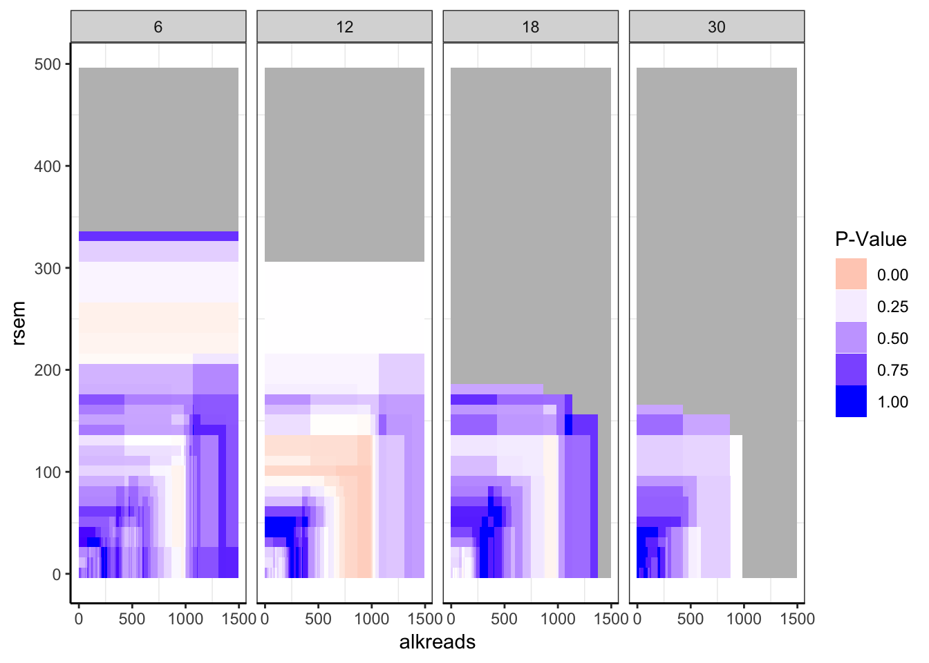
Expand here to see past versions of unnamed-chunk-8-5.png:
| Version | Author | Date |
|---|---|---|
| 4b082e4 | haiderinam | 2019-02-19 |
ALKATI vs BRAF
ALKATI is not mutually exclusive with BRAF across a range of filters
Heatmaps code continued P-values reported are the minimum p-values across RPKM filters Single heat map
datapoints=simresults %>%
  filter(rsem<=500,alkreads<=1500)%>%
  group_by(rsem,alkreads,tot_alk) %>%
  summarise(min_p_val_pc1=min(p_val_pc1),rpkm_atpval=rpkm[min(p_val_pc1)][1])
datapoints[datapoints$tot_alk<20,]$min_p_val_pc1=""
datapoints$min_p_val_pc1=as.numeric(datapoints$min_p_val_pc1)

  ggplot(datapoints,aes(x=alkreads,y=rsem))+geom_tile(aes(fill=min_p_val_pc1))+
      scale_fill_gradient2(low ="red" ,mid ="white" ,high ="blue",midpoint = .4 ,name="P-Value",na.value = "gray90",guide = "legend",breaks=c(.1,.2,.4,.6,.8,1))+
    # scale_fill_gradientn(colours =c("red", "white","blue"),values=c(0,.05,1),breaks=c(0,.05,.2,1),name="P-Value",na.value = "gray",guide = "legend")+
      theme(panel.grid.major = element_blank(),
            panel.grid.minor = element_blank(),
            panel.background = element_blank(),
            axis.line = element_line(colour = "black"))+
      xlab("Number of ALK Reads")+ylab("RSEM")+
      # ggtitle("Varying Combinations of Filters Does Not Create \nMutual Exclusivity Between ALK-ATI & BRAF")+
      theme_bw()+
      theme(plot.title = element_text(hjust=.5),text = element_text(size=30,face="bold"),axis.title = element_text(face="bold",size="26"),axis.text=element_text(face="bold",color="black",size="26"))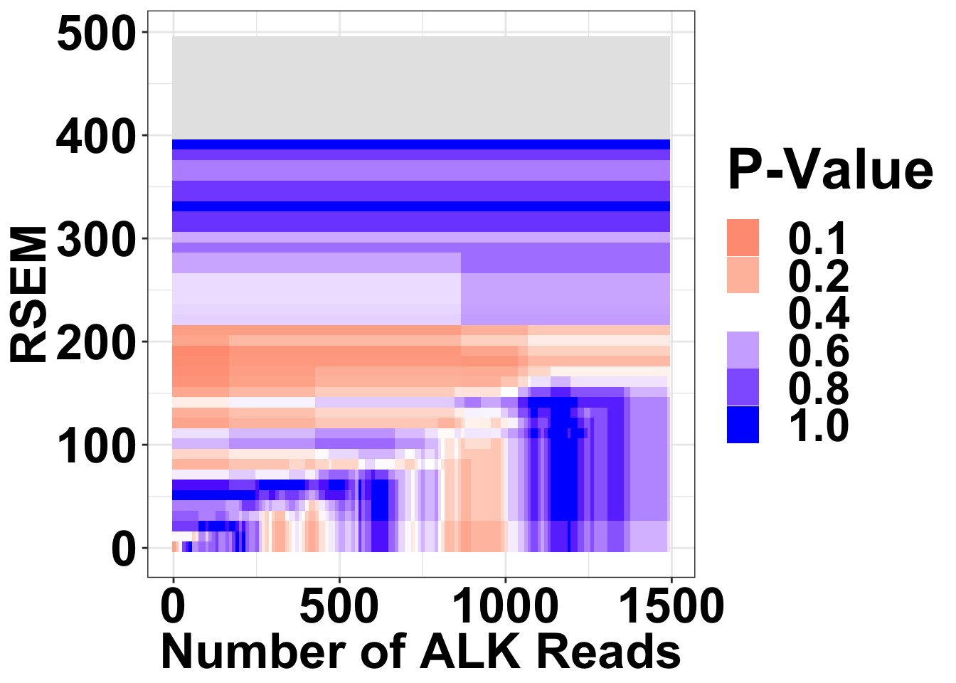
Expand here to see past versions of unnamed-chunk-9-1.png:
| Version | Author | Date |
|---|---|---|
| 0b5f5cb | haiderinam | 2019-02-19 |
| 4b082e4 | haiderinam | 2019-02-19 |
# ggsave("output/fig2b_filtercutoff_atibraf.pdf",width = 16,height = 14,units = "in",useDingbats=F)Facets of heat maps across a range of ex20-29/1-19 ratios
datapoints=simresults %>%
filter(rsem<=1000,alkreads<=2000,rpkm%in%c(6,12,18,30))%>%
group_by(rsem,alkreads,tot_alk,rpkm) %>%
summarise(min_p_val_pc1=min(p_val_pc1))

###Distribution of the number of ALKATI patients across different conditions
###Remember: ALKATI patients had exon ratio of 10, rsem >100, and counts >500. i.e. in the green region
###The takeaway from this plot is that we can try filters in the yellow region region. Will look at the p-values for these orange filters next

ggplot(datapoints,aes(x=alkreads,y=rsem))+geom_tile(aes(fill=tot_alk))+facet_grid(~rpkm)+
  scale_fill_gradientn(colours = rainbow(5),values=c(.1,.2,.3,.4,1),limits=c(0,100),breaks = c(9,10,20,30,40,100),name="# ALKATI \n Patients",guide = "legend")+
  ggtitle("Total ALKATI patients across exon20-29/ex1-19 ratios")+
  cleanup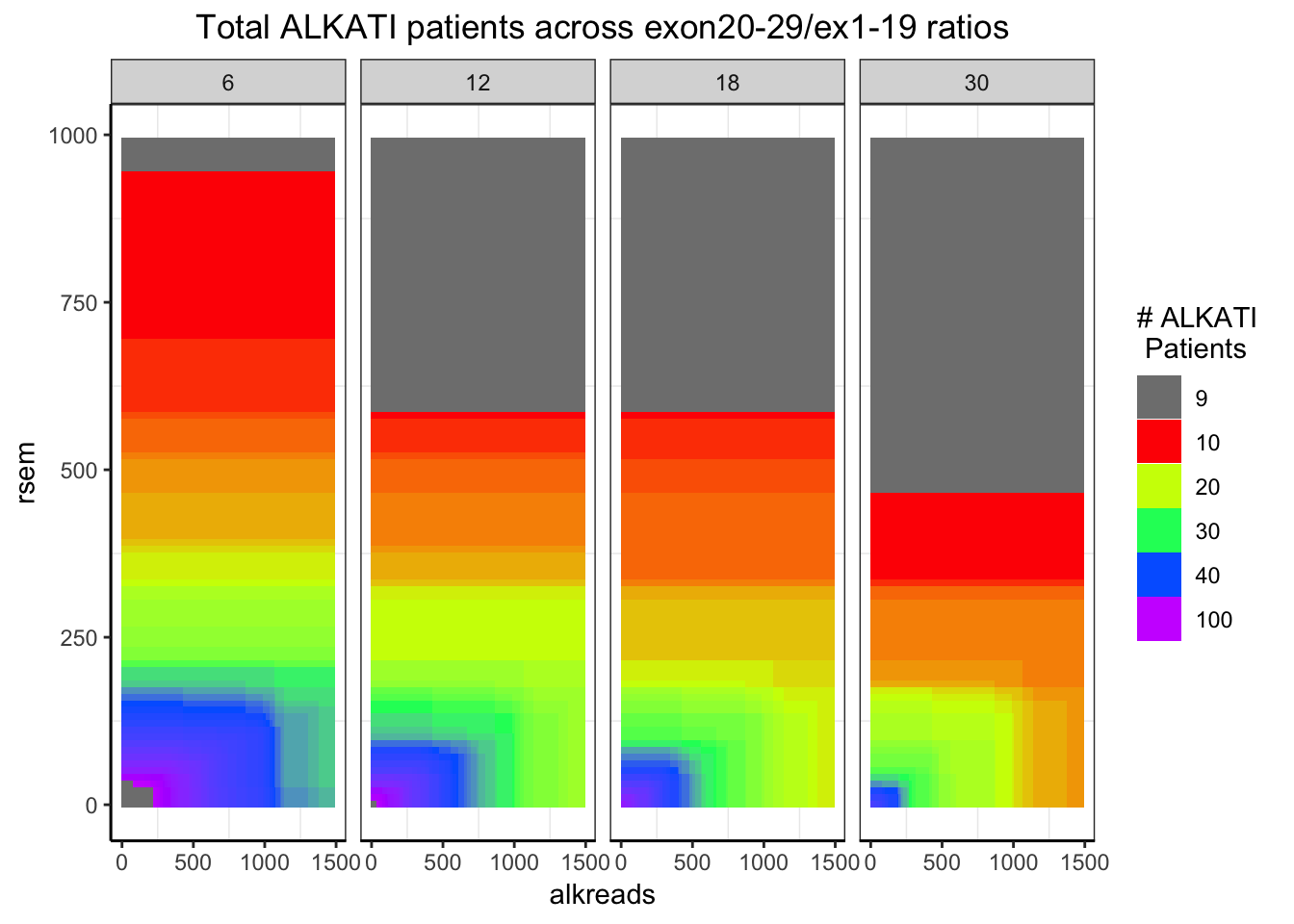
Expand here to see past versions of unnamed-chunk-10-1.png:
| Version | Author | Date |
|---|---|---|
| 4b082e4 | haiderinam | 2019-02-19 |
# P-Values Heat map
# Data is only plotted if number of ALKATI patients was >25
datapoints[datapoints$tot_alk<20,]$min_p_val_pc1=""
datapoints$min_p_val_pc1=as.numeric(datapoints$min_p_val_pc1)

ggplot(datapoints,aes(x=alkreads,y=rsem))+geom_tile(aes(fill=min_p_val_pc1))+facet_grid(~rpkm)+
  scale_fill_gradient2(low ="red" ,mid ="white" ,high ="blue",midpoint = .4 ,name="P-Value",guide = "legend",limits=c(0,1),na.value = "gray")+
  cleanup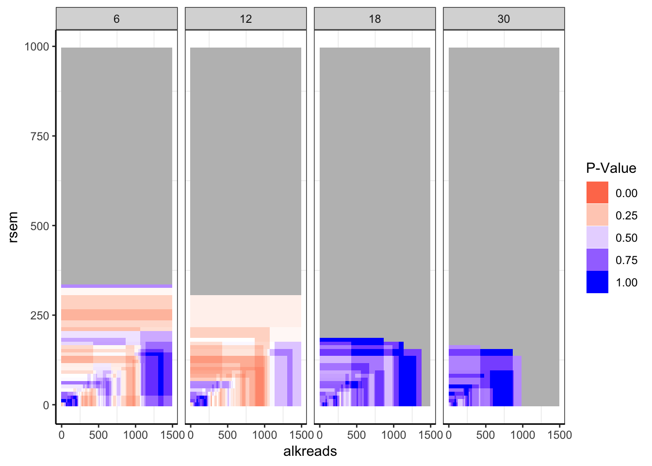
Expand here to see past versions of unnamed-chunk-10-2.png:
| Version | Author | Date |
|---|---|---|
| 4b082e4 | haiderinam | 2019-02-19 |
Session information
sessionInfo()R version 3.5.2 (2018-12-20)
Platform: x86_64-apple-darwin15.6.0 (64-bit)
Running under: macOS Mojave 10.14.3
Matrix products: default
BLAS: /Library/Frameworks/R.framework/Versions/3.5/Resources/lib/libRblas.0.dylib
LAPACK: /Library/Frameworks/R.framework/Versions/3.5/Resources/lib/libRlapack.dylib
locale:
[1] en_US.UTF-8/en_US.UTF-8/en_US.UTF-8/C/en_US.UTF-8/en_US.UTF-8
attached base packages:
[1] parallel stats graphics grDevices utils datasets methods
[8] base
other attached packages:
[1] bindrcpp_0.2.2 doParallel_1.0.14 iterators_1.0.10 foreach_1.4.4
[5] tictoc_1.0 dplyr_0.7.8 knitr_1.21 ggplot2_3.1.0
loaded via a namespace (and not attached):
[1] Rcpp_1.0.0 compiler_3.5.2 pillar_1.3.1
[4] git2r_0.24.0 plyr_1.8.4 workflowr_1.1.1
[7] bindr_0.1.1 R.methodsS3_1.7.1 R.utils_2.7.0
[10] tools_3.5.2 digest_0.6.18 evaluate_0.12
[13] tibble_2.0.1 gtable_0.2.0 pkgconfig_2.0.2
[16] rlang_0.3.1 yaml_2.2.0 xfun_0.4
[19] withr_2.1.2 stringr_1.3.1 rprojroot_1.3-2
[22] grid_3.5.2 tidyselect_0.2.5 glue_1.3.0
[25] R6_2.3.0 rmarkdown_1.11 reshape2_1.4.3
[28] purrr_0.3.0 magrittr_1.5 whisker_0.3-2
[31] codetools_0.2-16 backports_1.1.3 scales_1.0.0
[34] htmltools_0.3.6 assertthat_0.2.0 colorspace_1.4-0
[37] labeling_0.3 stringi_1.2.4 lazyeval_0.2.1
[40] munsell_0.5.0 crayon_1.3.4 R.oo_1.22.0 This reproducible R Markdown analysis was created with workflowr 1.1.1